Category Archives: Programming

Combining ray tracing and polygons

I have written a lot about distance estimated ray marching using OpenGL shaders on this blog.

But one of the things I have always left out is how to setup the camera and perspective projection in OpenGL. The traditional way to do this is by using functions such as ‘gluLookAt’ and ‘gluPerspective’. But things become more complicated if you want to combine ray marched shader graphics with the traditional OpenGL polygons. And if you are using modern OpenGL (the ‘core’ context), there is no matrix stack and no ‘gluLookAt’ functions. This post goes through through the math necessary to combine raytraced and polygon graphics in shaders. I have seen several people implement this, but I couldn’t find a thorough description of how to derive the math.

Here is the rendering pipeline we will be using:

It is important to point out, that in modern OpenGL there is no such thing as a model, view, or projection matrix. The green part on the diagram above is completely programmable, and it is possible to do whatever you like there. Only the part after the green box of the diagram (starting with clip coordinates) is fixed by the graphics card. But the goal here is to precisely match the convention of the fixed-function OpenGL pipeline matrices and the GLU functions gluLookAt and gluPerspective, so we will stick to the conventional model, view, and projection matrix terminology.

The object coords are the raw coordinates, for instance as specified in VBO buffers. This is the vertices of an 3D object in its local coordinate system. The next step is to position and orient the 3D object in the scene. This is accomplished by applying the model matrix, that transform the object coordinates to global world coordinates. The model transformation will be different for the different objects that are placed in the scene.

The camera transformation

The next step is to transform the world coordinates into camera or eye space. Now, neither old nor modern OpenGL has any special support for implementing a camera. Instead the conventional gluPerspective always assumes an origo centered camera facing the negative z-direction, and with an up-vector in the positive y-direction. So, in order to implement a generic, movable camera, we instead find a camera-view matrix, and then apply the inverse transformation to our world coordinates – i.e. instead of moving/rotate the camera, we apply the opposite transformation to the world.

Personally, I prefer using a camera specified using a forward, up, and right vector, and a position. It is easy to understand, and the only problem is that you need to keep the vectors orthogonal at all times. So we will use a camera identical to the one implemented in gluLookAt.

The camera-view matrix is then of the form:

\(
\begin{bmatrix}
r.x & u.x & -f.x & p.x \\
r.y & u.y & -f.y & p.y \\
r.z & u.z & -f.z & p.z \\
0 & 0 & 0 & 1
\end{bmatrix}
\)
 
where r=right, u=up, f=forward, and p is the position in world coordinates. R, u, and f must be normalized and orthogonal.

Which gives an inverse of the form:

\(
\begin{bmatrix}
r.x & r.y & r.z & q.x \\
u.x & u.y & u.z & q.y \\
-f.x & -f.y & -f.z & q.z \\
0 & 0 & 0 & 1
\end{bmatrix}
\)
 
By multiplying the matrices together and requiring the result is the identity matrix, the following relations between p and q can be established:

q.x = -dot(r,p), q.y = -dot(u,p), q.z = dot(f,p)
p = -vec3(vec4(q,0)*modelView); 

As may be seen, the translation part (q) of this matrix is the position of the camera expressed in the R,u, and f coordinate system.

Now, per default, the OpenGL shaders use a column-major representation of matrices, in which the data is stored sequentially as a series of columns (notice, that this can be changed by specifying ‘layout (row_major) uniform;’ in the shader). So creating the model-view matrix as an array on the CPU side looks like this:

float[] values = new float[] {
    r[0], u[0], -f[0], 0,
    r[1], u[1], -f[1], 0,
    r[2], u[2], -f[2], 0,
    q[0], q[1], q[2], 1};

Don’t confuse this with the original camera-transformation: it is the inverse camera-transformation, represented in column-major format.

The Projection Transformation

The gluPerspective transformation uses the following matrix to transform from eye coordinates to clip coordinates:

\(
\begin{bmatrix}
f/aspect & 0 & 0 & 0 \\
0 & f & 0 & 0 \\
0 & 0 & \frac{(zF+zN)}{(zN-zF)} & \frac{(2*zF*zN)}{(zN-zF)} \\
0 & 0 & -1 & 0
\end{bmatrix}
\)
 
where ‘f’ is cotangent(fovY/2) and ‘aspect’ is the width to height ratio of the output window.

(If you want to understand the form of this matrix, try this link)

Since we are going to raytrace the view frustum, consider what happens when we transform an direction of the form (x,y,-1,0) from eye space to clip coordinates and further to normalized device coordinates. Since the clip.w in this case will be 1, the x and y part of the NDC will be:

ndc.xy = (x*f/aspect, y*f)

Since normalized device coordinates range from [-1;1], this means that when we ray trace our frustrum, our ray direction (in eye space) must be in the range:

eyeX = [-aspect/f ; aspect/f] 
eyeY = [-1/f ; 1/f] 
eyeZ = -1

where 1/f = tangent(fovY/2).

We now have the necessary ingredients to set up our raytracing shaders.

The polygon shaders

But let us start with the polygon shaders. In order to draw the polygons, we need to apply the model, view, and projection transformations to the object space vertices:

gl_Position = projection * modelView * vertex;

Notice, that we premultiply the model and view matrix on the CPU side. We don’t need them individually on the GPU side. If you wonder why we don’t combine the projection matrix as well, it is because we want to use the modelView to transform the normals as well:

eyeSpaceNormal = mat3(modelView) * objectSpaceNormal; 

Notice, that in general normals transform different from positions. They should be multiplied by the inverse of the transposed 3×3 part of the modelView matrix. But if we only do uniform scaling and rotations, the above will work, since the rotational part of matrix is orthogonal, and the uniform scaling does not matter if we normalize our normals. But if you do non-uniform scaling in the model matrix, the above will not work.

The raytracer shaders

The raytracing must be done in world coordinates. So in the vertex shader for the raytracer, we need figure out the eye position and ray direction (both in world coordinates) for each pixel. Assume that we render a quad, with the vertices ranging from [-1,-1] to [1,1].

The eye position can be easily found from the formula found under ‘the camera transformation’:

eye = -(modelView[3].xyz)*mat3(modelView);

Similar, by transforming the ranges we found above from eye to world space we get that:

dir = vec3(vertex.x*fov_y_scale*aspect,vertex.y*fov_y_scale,-1.0)
	*mat3(modelView);

where fov_y_scale = tangent(fovY/2) is an uniform calculated on the CPU side.

Normally, OpenGL takes care of filling the z-buffer. But for raytracing, we have to do it manually, which can be done by writing to gl_fragDepth. Now, the ray tracing takes place in world coordinates: we are tracing from the eye position and into the camera-forward direction (mixed with camera-up and camera-right). But we need the z-coordinate of the hit position in eye coordinates. The raytracing is of the form:

vec3 hit = p + rayDirection * distance; // hit in world coords

Converting the hit point to eye coordinates gives (the p and q terms cancel):

eyeHitZ = -distance * dot(rayDirection * cameraForward);

which in clip coordinates becomes:

clip.z = [(zF+zN)/(zN-zF)]*eyeHitZ +  (2*zF*zN)/(zN-zF);
clip.w = -eyeHitZ;

Making the perspective divide, we arrive at normalized device coordinates:

ndcDepth = ((zF+zN) + (2*zF*zN)/eyeHitZ)/(zF-zN)

The ncdDepth is in the interval [-1;1]. The last step that remains is to convert into window coordinates. Here the depth value is mapped onto an interval determined by the gl_DepthRange.near and gl_DepthRange.far parameters (usually these are just 0 and 1). So finally we arrive at the following:

gl_FragDepth =((gl_DepthRange.diff * ndcDepth) + gl_DepthRange.near + gl_DepthRange.far) / 2.0;

Putting the pieces together, we arrive at the following for the ray tracing vertex shader:

void main(void)
{
  gl_Position = vertex;
  eye = -(modelView[3].xyz)*mat3(modelView);
  dir = vec3(vertex.x*fov_y_scale*aspect,vertex.y*fov_y_scale,-1.0)
			*mat3(modelView);
  cameraForward = vec3(0,0,-1.0)*mat3(modelView);
}

and this code for the fragment shader:

void main (void)
{
  vec3 rayDirection=normalize(dir);
  trace(eye,rayDirection, distance, color);
  fragColor = color;
  float eyeHitZ = -distance *dot(cameraForward,rayDirection);
  float ndcDepth = ((zFar+zNear) + (2.0*zFar*zNear)/eyeHitZ)
		/(zFar-zNear);
  gl_FragDepth =((gl_DepthRange.diff * ndcDepth) 
		+ gl_DepthRange.near + gl_DepthRange.far) / 2.0;
}

The above is of course just snippets. I’m currently experimenting with a Java/JOGL implementation of the above (Github repo), with some more complete code.
Optimizing GLSL Code

By making selected variables constant at compile time, some 3D fractals render more than four times faster. Support for easily locking variables has been added to Fragmentarium.

Some time ago, I became aware that the raytracer in Fragmentarium was somewhat slower than both Fractal Labs and Boxplorer for similar systems – this was somewhat puzzling since the DE raycasting technique is pretty much the same. After a bit of investigation, I realized that my standard raytracer had grown slower and slower, as new features had been added (e.g. reflections, hard shadows, and floor planes) – even if the features were turned off!

One way to speed up GLSL code, is by marking some variables constant at compile-time. This way the compiler may optimize code (e.g. unroll loops) and remove unused code (e.g. if hard shadows are disabled). The drawback is that changing these constant variables requires that the GLSL code is compiled again.

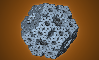
It turned out that this does have a great impact on some systems. For instance for the ‘Dodecahedron.frag’, take a look at the following render times:

No constants: 1.4 fps (1.0x)
Constant rotation matrices : 3.4 fps (2.4x)
Constant rotation matrices + Anti-alias + DetailAO: 5.6 fps (4.0x)
All 38 parameters (except camera): 6.1 fps (4.4x)

The fractal rotation matrices are the matrices used inside the DE-loop. Without the constant declarations, they must be calculated from scratch for each pixel, even though they are identical for all pixels. Doing the calculation at compile-time gives a notable speedup of 2.4x (notice that another approach would be to calculate such frame constants in the vertex shader and pass them to the pixel shader as ‘varying’ variables. But according to this post this is – surprisingly – not very effective).

The next speedup – from the ‘Anti-alias’ and ‘DetailAO’ variables – is more subtle. It is difficult to see from the code why these two variables should have such impact. And in fact, it turns out that combinations of other variables will amount in the same speedup. But these speedups are not additive! Even if you make all variables constants, the framerate only increases slightly above 5.6 fps. It is not clear why this happens, but I have a guess: it seems that when the complexity is lowered between a certain treshold, the shader code execution speed increases sharply. My guess is that for complex code, the shader runs out of free registers and needs to perform calculations using a slower kind of memory storage.

Interestingly, the ‘iterations’ variable offers no speedup – even though the compiler must be able to unroll the principal DE loop, there is no measurable improvement by doing it.

Finally, the compile time is also greatly reduced when making variables constant. For the ‘Dodecahedron.frag’ code, the compile time is ~2000ms with no constants. By making most variables constant, the compile time is lowered to around ~335ms on my system.

Locking in Fragmentarium.

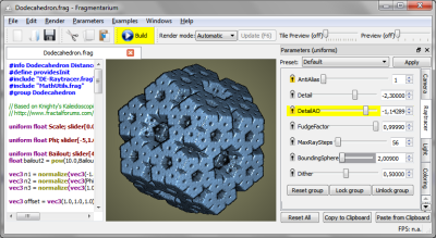
In Fragmentarium variables can be locked (made compile-time constant) by clicking the padlock next to them. Locked variables appear with a yellow padlock next to them. When a variable is locked, any changes to it will first be executed when the system is compiled (by pressing ‘build’). Locked variables, which have been changes, will appear with a yellow background until the system is compiled, and the changes are executed.

Notice, that whole parameter groups may be locked, by using the buttons at the bottom.

Screenshot

The locking interface – click to enlarge.


The ‘AntiAlias’ and ‘DetailAO’ variables are locked. The ‘DetailAO’ has been changed, but the changes are not executed yet (the yellow background). The ‘BoundingSphere’ variable has a grey background, because it has keyboard focus: its value can be finetuned using the arrow keys (up/down controls step size, left/right changes value).

In a fragment, a user variable can be marked as locked by default, by adding a ‘locked’ keyword to it:

uniform float Scale; slider[-5.00,2.0,4.00] Locked

Some variables can not be locked – e.g. the camera settings. It is possible to mark such variables by the ‘NotLockable’ keyword:

uniform vec3 Eye; slider[(-50,-50,-50),(0,0,-10),(50,50,50)] NotLockable

The same goes for presets. Here the locking mode can be stated, if it is different from the default locking mode:

#preset SomeName
AntiAlias = 1 NotLocked
Detail = -2.81064 Locked
Offset = 1,1,1
...
#endpreset

Locking will be part of Fragmentarium v0.9, which will be released soon.

GPU versus CPU for pixel graphics

After having gained a bit of experience with GPU shader programming during my Fragmentarium development, a natural question to ask is: how fast are these GPU’s?

This is not an easy question to answer, and it depends on the specific application. But I will try to give an answer for the kind of systems that I’m interested in: pixel graphics systems, where each pixel can be calculated independently of the others, such as raytraced 3D fractals.

Lets take my desktop computer, a fairly standard desktop machine, as an example. It is equipped with Nvidia Geforce 9800GT GPU @ 1.5 GHz, and a Intel Core 2 Quad Q8200 @ 2.33GHz.

How many processing unit are there?

Number of processing units (CPU): 4 CPU cores
Number of processing units (GPU): 112 Shader units

Based on these numbers, we might expect the GPU to be a factor of 28x times faster than the CPU. Of course, this totally ignores the efficiency and operating speed of the processing units. Lets try looking at the processing power in terms of maximum number of floating-point operations per second instead:

Theoretical Peak Performance

Both Intel and Nvidia list the GFLOPS (billion floating point operations per second) rating for their products. Intel’s list can be found here, and Nvidia’s here. For my system, I found the following numbers:

Performance (CPU): 37.3 GFLOPS
Performance (GPU): 504 GFLOPS

Based on these numbers, we might expect the GPU to be a factor of 14x times faster than the CPU. But what do these numbers really mean, and can they be compared? It turns out that these number are obtained by multiplying the processor frequency by the maximum number of instructions per clock cycle.

For the CPU, we have four cores. Now, when Intel calculate their numbers, they do it based on the special 128-bit SSE registers on every modern Pentium derived CPU. These extensions make it possible to handle two double precision floating point, or four single precision floating point numbers per clock cycle. And in fact there exists a special instruction – the MAD, or Multiply-Add, instruction – which allows for two arithmetic operations per clock cycle on each element in the SSE registers. These means Intel assume 4 (cores) x 2 (double precision floats) x 2 (MAD instructions) = 16 instructions per clock cycle. This gives the theoretical peak performance stated above:

Performance (CPU): 2.33 GHz * 4 * 2 * 2 = 37.3 GFLOPS (double precision floats)

What about the GPU? Here we have 112 independent processing units. On the GPU architecture an even more benchmarking-friendly instruction exists: the MAD+MUL which combines two multiplies and one addition in a single clock cycle. This means Nvidia assumes 112 (cores) * 3 (MAD+MUL instructions) = 336 instructions per clock cycle. Combining this with a stated processing frequency of 1.5 GHz, we arrive at the number stated earlier:

Performance (GPU): 1.5 GHz * 112 * 3 = 504 GFLOPS (single precision floats)

But wait… Nvidia’s number are for single precision floats – the Geforce 8800GT does not even support double precision floats. So for a fair comparison we should double Intel’s number, since the SSE extensions allows four simultaneous single precision numbers to be processed instead of two double precision floats. This way we get:

Performance (CPU): 2.33 GHz * 4 * 4 * 2 = 74.6 GFLOPS (single precision floats)

Now, using this as a guideline, we would expect my GPU to be a factor of 6.8x faster than my CPU. But we have some pretty big assumptions here: for instance, not many CPU programmers would write SSE-optimized code – and is a modern C++ compiler powerful enough to automatically take advantage of them anyway? And how often is the GPU able to use the three operation MUL+MAD instruction?

A real-world experiment

To find out I wrote a simple 2D Mandelbrot system and benchmarked it on the CPU and GPU. This is really the kind of computational tasks that I’m interested in: it is trivial to parallelize and is not memory-intensive, and the majority of executed code will be floating point arithmetics. I did not try to optimize the C++ code, because I wanted to see if the compiler was able to perform some SSE optimization for me. Here are the execution times:

13941 ms – CPU single precision (x87)
13941 ms – CPU double precision (x87)
10535 ms – CPU single precision (SSE)
11367 ms – CPU double precision (SSE)
424 ms – GPU single precision

(These numbers have some caveats – I did perform the tests multiple times and discarded the first few runs, but the CPU code was only single-threaded – so I assumed the numbers would scale perfectly and divided the execution times by four. Also, I verified by checking the generated assembly code, that SSE instructions indeed were used for the core Mandelbrot loop, when they were enabled.).

There are a couple of things to notice here: first, there is no difference between single and double precision on the CPU. This is as could be expected for the x87 compiled code (since the x87 defaults to 80-bit precision anyway), but for the SSE version, we would expect a double up in speed. As can be seen, the SSE code is really not very much more efficient the the x87 code – which strongly suggests that the compiler (here Visual Studio C++ 2008) is not very good at optimizing for SSE.

So for this example we got a factor of 25x speedup by using the GPU instead of the CPU.

“Measured” GFLOPS

Another questions is how this example compares to the theoretical peak performance. By using Nvidia’s Cg SDK I was able to get the GPU assembly code. Since I now could count the number of instruction in the main loop, and I knew how many iterations were performed, I was able to calculate the actual number of floating point operations per second:

GPU: 211 (Mandel)GFLOPS
CPU: 8.4 (Mandel)GFLOPS*

(*The CPU number was obtained by assuming the number of instructions in the core loop was the same as for the GPU: in reality, the CPU disassembly showed that the simple loop was partially unrolled to more than 200 lines of very complex assembly code.)

Compared to the theoretical maximum numbers of 504 GFLOPS and 74.6 GFLOPS respectively, this shows the GPU is much closer to its theoretical limit than the CPU.

GPU Caps Viewer – OpenCL

A second test was performed using the GPU Caps Viewer. This particular application includes a 4D Quaternion Julia fractal demo in OpenCL. This is interesting since OpenCL is a heterogeneous platform – it can be compiled to both CPU and GPU. And since Intel just released an alpha version of their OpenCL SDK, I could compare it to Nvidia’s SDK.

The results were interesting:

Intel OpenCL: ~5 fps
Nvidia OpenCL: ~35 fps

(The FPS did vary through the animation, so these numbers are not very accurate. There were no dedicated benchmark mode.)

This suggest that Intel’s OpenCL compiler is actually able to take advantage of the SSE instructions and provides a highly optimized output. Either that, or Nvidia’s OpenCL implementation is not very efficient (which is not likely).

The OpenCL based benchmark showed my GPU to be approximately 7x times faster than my CPU. Which is exactly the same as predicted by comparing the theoretical GFLOPS values (for single precision).

Conclusion

For normal code written in a high-level language like C or GLSL (multithreaded, single precision, and without explicit SSE instructions) the computational power is roughly equivalent to the number of cores or shader units. For my system this makes the GPU a factor of 25x faster.

Even though the CPU cores have higher operating frequency and in principle could execute more instructions via their SSE registers, this does not seem be fully utilized (and in fact, compiling with and without SSE optimization did not make a significant difference, even for this very simple example).

The OpenCL example tells another story: here the measured performance was proportional to the theoretical GFLOPS ratings. This is interesting since this indicate, that OpenCL could also be interesting for CPU-applications.

One thing to bear in mind is, that the examples tested here (the Mandelbrot and 4D Quaternion Julia) are very well-suited for GPU execution. For more complex code, with conditional branching, double precision floating point operations, and non-coalesced memory access, the CPU is much more efficient than the GPU. So for a desktop computer such as mine, a factor of 25x is probably the best you can hope for (and it is indeed a very impressive speedup for any kind of code).

It is also important to remember that GPU’s are not magical devices. They perform operations with a theoretical peak performance typically 5-15 times larger than a CPU. So whenever you see these 1000x speed up claims (e.g. some of the CUDA showcases), it is probably just an indication of a poor CPU implementation.

But even though the performance of GPU’s may be somewhat exaggerated you can still get a tremendous speedup. And GPU interfaces such as GLSL shaders are really simple to use: you do not need to deal explicitly with threads, you have built-in vectors and matrices, and you can compile GLSL code dynamically, during run-time. All features which makes GPU programming nearly ideal for exploring pixel graphic systems.

Creating a Raytracer for Structure Synth (Part II)

When I decided to implement the raytracer in Structure Synth, I figured it would be an easy task – after all, it should be quite simple to trace rays from a camera and check if they intersect the geometry in the scene.

And it turned out, that it actually is quite simple – but it did not produce very convincing pictures. The Phong-based lighting and hard shadows are really not much better than what you can achieve in OpenGL (although the spheres are rounder). So I figured out that what I wanted was some softer qualities to the images. In particular, I have always liked the Ambient Occlusion and Depth-of-field in Sunflow. One way to achieve this is by shooting a lot of rays for each pixel (so-called distributed raytracing). But this is obviously slow.

So I decided to try to choose a smaller subset of samples for estimating the ambient occlusion, and then do some intelligent interpolation between these points in screen space. The way I did this was to create several screen buffers (depth, object hit, normal) and then sample at regions with high variations in these buffers (for instance at every object boundary). Then followed the non-trivial task of interpolating between the sampled pixels (which were not uniformly distributed). I had an idea that I could solve this by relaxation (essentially iterative smoothing of the AO screen buffer, while keeping the chosen samples fixed) – the same way the Laplace equation can be numerically solved.

While this worked, it had a number of drawbacks: choosing the condition for where to sample was tricky, the smoothing required many steps to converge, and the approach could not be easily multi-threaded. But the worst problem was that it was difficult to combine with other stuff, such as anti-alias and depth-of-field calculations, so artifacts would show up in the final image.

I also played around with screen based depth-of-field. Again I thought it would be easy to apply a Gaussian blur based on the z-buffer depth (of course you have to prevent background objects from blurring the foreground, which complicates things a bit). But once again, it turned out that creating a Gaussian filter for each particular depth actually gets quite slow. Of course you can bin the depths, and reuse the Gaussian filters from a cache, but this approach got complicated, and the images still displayed artifacts. And a screen based method will always have limitations: for instance, the blur from an object hidden behind another object will never be visible, because the object is not part of the screen buffers.

So in the end, I ended up discarding all the hacks, and settled for the much more satisfying solution of simply using a lot of rays for each pixel.

This may sound very slow: after all you need multiple rays for anti-alias, multiple rays for depth-of-field, multiple rays for ambient occlusion, for reflections, and so forth, which means you might end up with a combinatorial explosion of rays per pixel. But in practice there is a nice shortcut: instead of trying all combinations, just choose some random samples from all the possible combinations.

This works remarkably well. You can simulate all these complex phenomena with a reasonably number of rays. And you can use more clever sampling strategies in order to reduce the noise (I use stratified sampling in Structure Synth). The only drawback is, that you need a bit of book-keeping to prepare your stratified samples (between threads) and ensure you don’t get coherence between the different dimensions you sample.

Another issue was how to accelerate the ray-object intersections. This is a crucial part of all raytracers: if you need to check your rays against every single object in the scene, the renders will be extremely slow – the rendering time will be proportional to the number of objects. On the other hand spatial acceleration structures are often able to render a scene in a time proportional to the logarithm of the number of objects.

For the raytracer in Structure Synth I chose to use a uniform grid (aka voxel stepping). This turned out to be a very bad choice. The uniform grid works very well, when the geometry is evenly distributed in the scene. But for recursive systems, objects in a scene often appear at very different scales, making the cells in the grid very unevenly populated.

Another example of this is, that I often include a ground plane in my Structure Synth scenes (by using a flat box, such as “{ s 1000 1000 0.1 } box”). But this will completely kill the performance of the uniform grid – most objects will end up in the same cell in the grid, and the acceleration structure gets useless. So in general, for generative systems with different scales, the use of a uniform grid is a bad choice.

Not that is a lot of stuff, that didn’t work out well. So what is working?

As of now the raytracer in Structure Synth provides a nice foundation for things to come. I’ve gotten the multi-threaded part set correctly up, which includes a system for coordinating stratified samples. Each thread have its own (partial) screen space buffer, which means I can do progressive rendering. This also makes it possible to implement more complex filtering (where the filtered samples may contribute to more than one pixel – in which case the raytracer is not embarrassingly parallel anymore).

What is missing?

Materials. As of now there is only very limited control of materials. And things like transparency doesn’t work very well.

Filtering. As I mentioned above, the multi-threaded renderer supports working with filters, but I haven’t included any filters in the latest release. My first experiments (with a Gaussian filter) were not particularly successful.

Lighting. As of now the only option is a single, white, point-like light source casting hard shadows. This rarely produce nice pictures.

In the next post I’ll talk a bit about what I’m planning for future versions of the raytracers.

Cinder – Creative Coding in C++

Cinder is a new C++ library for creative applications. It is free, open-source, and cross-platform (Windows, Mac, iPhone/iPad, but no Linux). Think of it as Processing, but in C++.

Cinder offers classes for image processing, matrix, quaternion, spline and vector math, but also more general stuff like XML, HTTP, IO, and 2D Graphics.

The more generic stuff is implemented via third-party libraries, such as TinyXML, Cairo, AntTweakBar (a simple GUI), Boost (smart pointers and threads) and system libraries (QuickTime, Cocoa, DirectAudio, OpenGL) – certainly an ambitious range of technologies and uses.

Their examples are impressive, especially some of the demos by Robert Hodgin (flight404):


Cymatic Ferrofluid by flight404 (be sure to watch the videos).

Robert Hodgin has also created a very nice Cinder tutorial, which guides you through the creation of a quite spectacular particle effect.

Finally, it should be noted the openFrameworks offers related functionality, also based on C++.

Assorted Links

Generative Music Software

Adam M. Smith has begun working on cfml – a context-free music language. It is a Context-Free Design Grammar – for music. I’m very interested in how this develops.


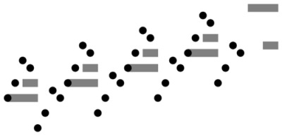
A graphical representation of cfml output (original here)

Cfml is implemented as an Impromptu library. Impromptu is a live coding environment, based on the Scheme language, and has existed since 2005. Andrew Sorensen, the developer of Impromptu, has created some of the most impressive examples of live coding I have seen. In particular, the last example, inspired by Keith Jarrett’s Sun Bear Concerts, is really impressive. (I might be slightly biased here, since I believe that Jarrett’s solo piano concerts – especially the Köln Concert and the Sun Bear Concerts – rank among the best music ever made).

Finally, Supercollider 140 is a selection of audio pieces all created in Supercollider in 140 characters or less. An interesting example of using restrictions to spur creativity. Another example is the 200 char Processing sketch contest.

Free Indy Game Development

This month also saw the release of the Unreal Development Kit, basically a version of the Unreal Engine 3, that is free for non-commercial use. This is great news for amateur game developers, but for me, the big question was whether this could be used as a powerful platform for generative art or live demos. I downloaded the kit and played around with it for a while, but while the 3D engine is stunning, UDK seems very geared towards graphical development (I certainly do not want to do draw my programs, and the built-in Unrealscript does not impress me either).

In related news, that basic version of Unity 2.6 is now also free. The main focus of Unity is also game development, but from a generative art / live demo perspective it holds greater promise. Unity offers an advanced graphics engine with user-scriptable shaders, integrated PhysX physics engine, and 3D audio.

Unitys development architecture is also very solid: scripts are written in (JIT-compiled) JavaScript, and components can be written in C# (using Mono, the open-source .NET implementation). Using a dynamic scripting language such as JavaScript to control a more rigid body of classes written in a more strict, statically typed environment, such as C#, is a good way to manage complex software. All Mozilla software – including Firefox – is built using this model (JavaScript + XPCOM C++ components), and newer platforms, such as Microsoft’s Silverlight platform also use it (JavaScript + C# components).

I made a few tests with Unity, and it is simple to control and instance even pretty complex structures. I considered writing a simple Structure Synth viewer using Unity, but was unfortunately put a bit off, when I discovered that Screen Space Ambient Occlusion and Full Screen Post-Processing Effects are not part of the free basic edition. The iPhone version of the Unity engine is not free either, but that is probably as could be expected.

It will be interesting to see if Unity will be picked up by the Generative Art community.

SIGGRAPH Asia

Finally two papers presented at SIGGRAPH Asia 2009 should be noted:

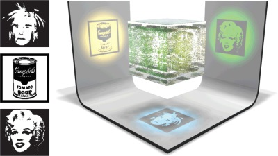
Shadow Art creates objects which cast three different shadows.

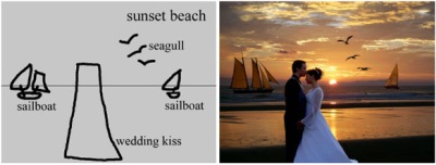
Sketch2Photo creates realistic photo-montages from freehand sketches annotated with text labels.

Random Colors, Color Pools, and Dual Mersenne Twister Goodness.

I’ve implemented a random color scheme in Structure Synth, using a new ‘color random’ specifier.

But what exactly is a random color? My first attempt was to use the HSV color model and choose a random hue, with full brightness and saturation.

This produces colors like this:

Most of my Nabla pictures used this color scheme. It produces some very strong colors.

Then I tried the RGB model using 3 random numbers, one for each color-channel, which creates this kind of colors:

But what about greyscale colors:

I decided that it was necessary to be able to switch between different color schemes.

So I created a new ‘set colorpool’ command. Besides the color schemes above (‘set colorpool randomhue’, ‘set colorpool randomrgb’, and ‘set colorpool greyscale’) I created two additional color schemes:

One where you specify a list of colors:

(For this image the command was: “set colorpool list:orange,white,white,white,white,white,white,grey”. As is evident it is possible to repeat a given color, to emphasize its occurrence in the image.)

And on where you specify an image which is used to sample colors from:

The command used for the above image was: “set colorpool image:001.PNG”. Whenever a random color is requested (by the ‘random color’ operator), the program will sample a random point from the specified image and use the color of this pixel. This is a quite powerful command, making it possible to imitate the color tonality of another picture.

Now this is all good. But I realized that there are some problems with this approach.

The problem is that geometry and the colors draw numbers from the same random number generator (the C-standard library ‘rand()’ function).

This means that changing the color scheme changes the geometry (since the color schemes use a different number of random numbers for each color – randomhue uses 1 random number per color, the image sampling uses two (X and Y) random numbers per color, the randomrgb uses three).

This is not acceptable, since you’ll want to change the color schemes without changing the geometry. Another problem is that C-standard library ‘rand’ function is not platform independent – so even if you specify a EisenScript together with an initial random seed, you will not get the same structure on different platforms.

I solved this by implementing new random generators in Structure Synth. I now use two independent Mersenne Twister random number generators, so that I have two random streams – one for geometry and one for colors.

The Second Coming of JavaScript

Some months ago, John Resig created processing.js – an impressive JavaScript port of processing, which draws its output on a ‘canvas’ element entirely client-side inside your browser (at least if your web-browser is Firefox 3 or a recent nightly build of WebKit, that is).

Now Context Free (the original inspiration for Structure Synth) has been ported to JavaScript too: Aza Raskin has created ContextFree.js (Source here).

JavaScript has undergone a tremendous evolution. From creating cheesy ‘onMouseOver’ effects for buttons on web pages to being the ‘glue’ binding together complex applications like Firefox or Songbird (the Mozilla application frameworks works by stringing together C++ components with JavaScript). Likewise Microsoft chose to build their Silverlight technology on .NET components which can be controlled by JavaScript in the browser.

And of course the ActionScript in Adobe Flash is also JavaScript. Adobe (and/or Macromedia) has put a lot of effort into creating fast JavaScript implementations – most notably their Tamarin virtual machine and Just-In-Time compiler, which in theory should make JavaScript almost as fast as native code – or at least comparable to other JIT compiled languages such as Java and the .NET languages. Tamarin is open-sourced, and will eventually make it into Firefox 4.

Finally, while the Tamarin virtual machine was built to execute (and JIT) bytecode originating from JavaScript, other languages may target Tamarin as well. Adobe has demonstrated the possibility of compiling standard C programs into Tamarin parseable byte-code (their demo included Quake, a Nintendo emulator, and several languages like Python and Ruby).

So perhaps a future version of Structure Synth could be running as C++ compiled into Tamarin bytecode in a Flash application…

Underground code

The Demo Scene never cease to amaze me. The technical quality of these demos is amazing – complex 3D scenes rendered real-time, procedural textures, real-time sound synthesis, and incredible low foot-prints.

Recently I stumbled upon demoscene.tv which features recorded videos (flash video) of many of the best demos. Of course part of the fun is actually running these demos, to be amazed that they are indeed real-time, but sadly my laptop is not geared towards neither CPU or GPU intensive activities.

A few selected demos:


fr-041: debris by Farbrausch


Lifeforce by andromeda software development