The previous posts (part I, part II) introduced the basics of rendering DE (Distance Estimated) systems, but left out one important question: how do we create the distance estimator function?

Drawing spheres

Remember that a distance estimator is nothing more than a function, that for all points in space returns a length smaller than (or equal to) the distance to the closest object. This means we are safe to march at least this step length without hitting anything – and we use this information to speed up the ray marching.

It is fairly easy to come up with distance estimators for most simple geometric shapes. For instance, let us start by a sphere. Here are three different ways to calculate the distance from a point in space, p, to a sphere with radius R:

(1) DE(p) = max(0.0, length(p)-R)  // solid sphere, zero interior
(2) DE(p) = length(p)-R // solid sphere, negative interior
(3) DE(p) = abs(length(p)-R)    // hollow sphere shell

From the outside all of these look similar. But (3) is hollow – we would be able to position the camera inside it, and it would look different if intersected with other objects.

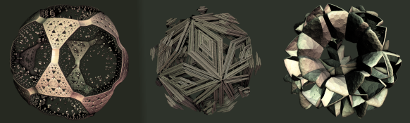
What about the first two? There is actually a subtle difference: the common way to find the surface normal, is to sample the DE function close to the camera ray/surface intersection. But if the intersection point is located very close to the surface (for instance exactly on it), we might sample the DE inside the sphere. And this will lead to artifacts in the normal vector calculation for (1) and (3). So, if possible use signed distance functions. Another way to avoid this, is to backstep along the camera ray a bit before calculating the surface normal (or to add a ray step multiplier less than 1.0).

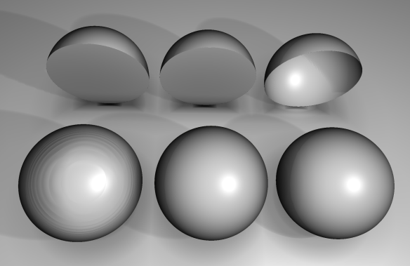
From left to right: Sphere (1), with normal artifacts because the normal was not backstepped. Sphere (2) with perfect normals. Sphere (3) drawn with normal backstepping, and thus perfect normals. The last row shows how the spheres look when cut open.

Notice that distance estimation only tells the distance from a point to an object. This is in contrast to classic ray tracing, which always is about finding the distance from a point to a given object along a line. The formulas for ray-object intersection in classic ray tracing are thus more complex, for instance the ray-sphere intersection involves solving a quadratic equation. The drawback of distance estimators is that multiple ray steps are needed, even for simple objects like spheres.

Combining objects

Distance fields have some nice properties. For instance, it is possible to combine two distance fields using a simple minimum(a,b) operator. As an example we could draw the union of two spheres the following way:

DE(p) = min( length(p)-1.0 , length(p-vec3(2.0,0.0,0.0))-1.0 );

This would give us two spheres with unit radius, one centered at origo, and another at (2,0,0). The same way it is possible to calculate the intersection of two objects, by taking the maximum value of the fields. Finally, if you are using signed distance functions, it is possible to subtract one shape from another by inverting one of the fields, and calculating the intersection (i.e. taking max(A, -B)).

So now we have a way to combine objects. And it is also possible to apply local transformations, to get interesting effects:

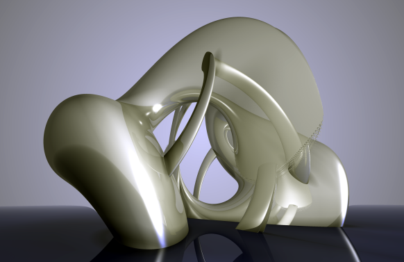
This image was created by combining the DE’s of a ground plane and two tori while applying a twisting deformation to the tori.

Rendering of (non-fractal) distance fields is described in depth in this paper by Hart: Sphere Tracing: A Geometric Method for the Antialiased Ray Tracing of Implicit Surfaces. This paper also describes distance estimators for various geometric objects, such as tori and cones, and discuss deformations in detail. Distance field techniques have also been adopted by the demoscene, and Iñigo Quilez’s introduction contains a lot of information. (Update: Quilez has created a visual reference page for distance field primitives and transformations)

Building Complexity

This is all nice, but even if you can create interesting structures, there are some limitations. The above method works fine, but scales very badly when the number of distance fields to be combined increases. Creating a scene with 1000 spheres by finding the minimum of the 1000 fields would already become too slow for real-time purposes. In fact ordinary ray tracing scales much better – the use of spatial acceleration structures makes it possible for ordinary ray tracers to draw scenes with millions of objects, something that is far from possible using the “find minimum of all object fields” distance field approach sketched above.

But fractals are all about detail, and endless complexity, so how do we proceed?

It turns out that there are some tricks, that makes it possible to add complexity in ways that scales much better.

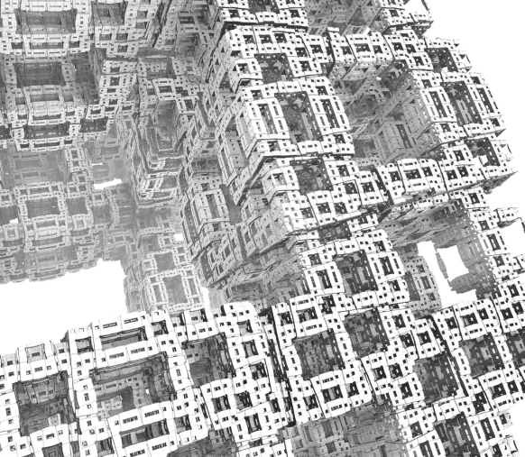
First, it is possible to reuse (or instance) objects using e.g. the modulo-operator. Take a look at the following DE:

float DE(vec3 z)
{
  z.xy = mod((z.xy),1.0)-vec3(0.5); // instance on xy-plane
  return length(z)-0.3;             // sphere DE
}

Which generates this image:

Now we are getting somewhere. Tons of detail, at almost no computational cost. Now we only need to make it more interesting!

A Real Fractal

Let us continue with the first example of a real fractal: the recursive tetrahedron.

A tetrahedron may be described as a polyhedron with vertices (1,1,1),(-1,-1,1),(1,-1,-1),(-1,1,-1). Now, for each point in space, lets us take the vertex closest to it, and scale the system by a factor of 2.0 using this vertex as center, and then finally return the distance to the point where we end, after having repeated this operation. Here is the code:

float DE(vec3 z)
{
	vec3 a1 = vec3(1,1,1);
	vec3 a2 = vec3(-1,-1,1);
	vec3 a3 = vec3(1,-1,-1);
	vec3 a4 = vec3(-1,1,-1);
	vec3 c;
	int n = 0;
	float dist, d;
	while (n < Iterations) {
		 c = a1; dist = length(z-a1);
	        d = length(z-a2); if (d < dist) { c = a2; dist=d; }
		 d = length(z-a3); if (d < dist) { c = a3; dist=d; }
		 d = length(z-a4); if (d < dist) { c = a4; dist=d; }
		z = Scale*z-c*(Scale-1.0);
		n++;
	}

	return length(z) * pow(Scale, float(-n));
}

Which results in the following image:

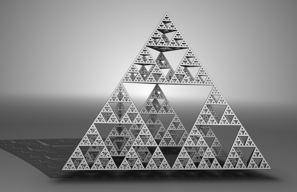
Our first fractal! Even though we do not have the infinite number of objects, like the mod-example above, the number of objects grow exponentially as we crank up the number of iterations. In fact, the number of objects is equal to 4^Iterations. Just ten iterations will result in more than a million objects - something that is easily doable on a GPU in realtime! Now we are getting ahead of the standard ray tracers.

Folding Space

But it turns out that we can do even better, using a clever trick by utilizing the symmetries of the tetrahedron.

Now, instead of scaling about the nearest vertex, we could use the mirror points in the symmetry planes of the tetrahedron, to make sure that we arrive at the same "octant" of the tetrahedron - and then always scale from the vertex it contains.

The following illustration tries to visualize this:

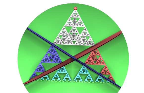
The red point at the top vertex is the scaling center at (1,1,1). Three symmetry planes of the tetrahedron have been drawn in red, green, and blue. By mirroring points if they are on the wrong side (the non-white points) of plane, we will ensure they get mapped to the white "octant". The operation of mirroring a point, if it is on one side of a plane, is called a 'folding operation' or just a fold.

Here is the code:

float DE(vec3 z)
{
    float r;
    int n = 0;
    while (n < Iterations) {
       if(z.x+z.y<0) z.xy = -z.yx; // fold 1
       if(z.x+z.z<0) z.xz = -z.zx; // fold 2
       if(z.y+z.z<0) z.zy = -z.yz; // fold 3	
       z = z*Scale - Offset*(Scale-1.0);
       n++;
    }
    return (length(z) ) * pow(Scale, -float(n));
}

These folding operations shows up in several fractals. A fold in a general plane with normal n can be expressed as:

float t = dot(z,n1); if (t<0.0) { z-=2.0*t*n1; }

or in a optimized version (due to AndyAlias):

z-=2.0 * min(0.0, dot(z, n1)) * n1;

Also notice that folds in the xy, xz, or yz planes may be expressed using the 'abs' operator.

That was a lot about folding operations, but the really interesting stuff happens when we throw rotations into the system. This was first introduced by Knighty in the Fractal Forum's thread Kaleidoscopic (escape time) IFS. The thread shows recursive versions of all the Platonic Solids and the Menger Sponge - including the spectacular forms that arise when inserting rotations and translations into the system.

The Kaleidoscopic IFS fractals are in my opinion some of the most interesting 3D fractals ever discovered (or created if you are not a mathematical platonist). Here are some examples of forms that may arise from a system with icosahedral symmetry:

Here the icosahedral origin might be evident, but it possible to tweak these structures beyond any recognition of their origin. Here are a few more examples:

Knighty's fractals are composed using a small set of transformations: scalings, translations, plane reflections (the conditional folds), and rotations. The folds are of course not limited to the symmetry planes of the Platonic Solids, all planes are possible.

The transformations mentioned above all belong to the group of conformal (angle preserving) transformations. It is sometimes said (on Fractal Forums) that for 'true' fractals the transformations must be conformal, since non-conformal transformations tend to stretch out detail and create a 'whipped cream' look, which does not allow for deep zooms. Interestingly, according to Liouville's theorem there are not very many possible conformal transformations in 3D. In fact, if I read the theorem correctly, the only possible conformal 3D transformations are the ones above and the sphere inversions.

Part IV discusses how to arrive at Distance Estimators for the fractals such as the Mandelbulb, which originates in attempts to generalize the Mandelbrot formula to three dimensions: the so-called search for the holy grail in 3D fractals.